In the four crashes studied (2000, 2008, 2020 and 2022), no asset class protected every time: government bonds gained over the 2000 and 2008 windows but fell 19.9% to 21.2% at worst in the 2022 rate shock (December 2020 to December 2024), while gold in euros never fell more than 13.3% within a crisis window.
This study measures, in euros, the maximum drawdown (max. loss), the three-year return and the recovery time of 15 index series during four crises: the dot-com bubble (2000), the financial crisis (2008), Covid (2020) and the inflation and interest-rate shock (2022). The reported summary tables can be downloaded at the end of the article.
The comparison objective here is compounded wealth after costs. Drawdown, recovery time and correlation describe the path; lower volatility or more diversification alone does not establish better growth. Four selected crisis windows cannot identify a portfolio that maximises future geometric growth.
Key takeaways
- Government bonds had positive window returns in the selected 2000 and 2008 episodes, but losses in the later rate shock. Euro government bonds lost 3.5% at worst over the 2008 crisis window, against 53.7% for European equities, but lost 21.2% between December 2020 and December 2022.
- Spreading equities across regions and holding high-yield bonds did not protect against the 2008 crisis. Across the six equity series displayed below, maximum month-end losses ranged from 39.8% to 56.4% during September 2007–September 2010; euro high-yield bonds lost 34.2% within that window.
- Gold in euros limited its losses in all four crises, but gold is not risk-free over the long term. The maximum drawdown of gold in euros stayed between 8.8% and 13.3% in each crisis window, yet gold in euros spent 24 years and 8 months below its January 1983 peak.
- Depth and duration describe different parts of the wealth path. The S&P 500 in euros, dividends reinvested, took 13 years and 3 months to regain its August 2000 peak, and Japanese equities almost 18 years to regain their March 2000 peak.
- Displayed equity series: maximum month-end losses of 49.1%–66.7% in February 2000–February 2003 and 39.8%–56.4% in September 2007–September 2010. These are selected indices, not every equity market.
- Government bonds: maximum month-end losses of 1.6%–3.5% across the two displayed series and the 2000 and 2008 windows, then -21.2% for euro government bonds in the 2020-2022 rate shock.
- Gold in euros: maximum drawdown between 8.8% and 13.3% in all four crises, and +82.8% over the 2008 crisis window.
- High yield: -34.2% within September 2007–September 2010, while its full-window return was +13.6%. Credit exposure can produce large interim losses despite bond income.
- Recovery: 13 years and 3 months for the S&P 500 in euros after its August 2000 peak, almost 18 years for Japanese equities, more than 24 years for gold after its 1983 peak.
Figures without an external link are Copio calculations from archived index levels, at month-end in euros. Reproduction and source limits appear above and in the methodology.
The four crashes in one table
Maximum drawdown (peak to trough, month-end values, in euros) and cumulative index return over each crisis's three-year window. Return conventions differ by index; these are not uniformly net investor total returns.
| Asset class | Dot-com bubble (2000-2003) | 2008 crisis (2007-2010) | Covid (2020-2023) | Rate shock (2021-2024) |
|---|
| US equities (S&P 500, dividends reinvested) | -52.5% / -42.1% | -44.1% / -16.9% | -18.9% / +35.4% | -13.0% / +41.0% |
| European equities (STOXX Europe 600) | -51.9% / -50.2% | -53.7% / -24.5% | -21.6% / +18.2% | -18.6% / +12.6% |
| French equities (CAC 40, dividends reinvested) | -56.4% / -52.6% | -51.7% / -26.8% | -24.1% / +31.7% | -17.1% / +13.1% |
| German equities (DAX) | -66.7% / -66.7% | -52.4% / -20.8% | -23.7% / +16.5% | -23.7% / +25.3% |
| Japanese equities (MSCI Japan IMI) | -63.8% / -60.5% | -39.8% / -22.9% | -15.6% / +5.6% | -13.4% / +17.5% |
| Emerging-market equities (MSCI EM IMI) | -49.1% / -48.2% | -56.4% / +1.0% | -21.7% / +8.9% | -18.6% / +4.5% |
| Euro government bonds | -2.1% / +26.8% | -3.5% / +20.7% | -21.2% / -17.4% | n/a |
| Global government bonds (EUR-hedged) | -1.6% / +27.5% | -2.1% / +20.2% | -18.1% / -14.0% | -17.3% / -12.4% |
| Euro corporate bonds | n/a | -5.0% / +21.3% | -16.8% / -12.5% | -15.2% / -3.8% |
| Euro high-yield bonds | n/a | -34.2% / +13.6% | -15.0% / -2.4% | -13.6% / +8.2% |
| Euro inflation-linked bonds | n/a | -6.4% / +18.6% | -12.2% / -1.2% | -12.2% / -4.2% |
| Gold (in euros) | -10.5% / +6.6% | -12.5% / +82.8% | -13.3% / +23.9% | -8.8% / +56.4% |
| Commodities | -16.7% / +27.4% | -40.3% / -2.7% | -13.3% / +80.5% | -18.4% / +28.9% |
| Euro cash (money market) | 0.0% / +12.6% | 0.0% / +6.2% | -1.2% / -0.7% | -0.3% / +7.5% |
| Listed real estate (FTSE EPRA Nareit Developed) | n/a | n/a | n/a | -25.7% / -6.1% |
How to read it: maximum drawdown / total return over the window. n/a: series not available for the window. Windows: February 2000 - February 2003, September 2007 - September 2010, January 2020 - January 2023, December 2021 - December 2024. Because the windows are fixed, some declines continue beyond them (measured from its August 2000 peak, the S&P 500 in euros did not hit its low until February 2009, at -60.2%).
2008 versus 2022: different bond and equity outcomes
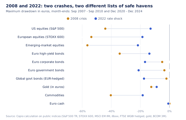
The chart measures the rate shock from December 2020 to December 2024, or the end of each available series. This captures bond peaks before 2022. The table above uses December 2021 to December 2024, so some drawdowns differ.
The episodes illustrate different interest-rate and growth conditions; the table alone cannot isolate their causes.
- 2000 and 2008 windows: the two government-bond series had positive cumulative returns. Falling required yields can raise the present value of fixed payments, but duration, credit, income and currency exposure also affect returns. Commodities returned +27.4% in the 2000–2003 window, so it would be wrong to say every growth-sensitive asset fell throughout both windows.
- Later rate shock: the euro-government-bond summary records a 21.2% drawdown from December 2020 to December 2022. The global EUR-hedged government series fell 20.2% from July 2020 to October 2023 and had not regained its July 2020 peak by April 2026, its available endpoint. These are different series and windows, not interchangeable estimates of a calendar-2022 loss.
This shift matches the change of sign in the correlation between stocks and bonds, analysed in our article on diversification.
How long does it take to regain the previous peak?
The worst observed decline of each displayed index over its available history, in euros, and the time spent below the previous peak.
| Asset class (history) | Worst decline | Peak | Trough | Peak regained | Time below peak |
|---|
| Gold in euros (1970-2026) | -54.0% | January 1983 | July 1999 | September 2007 | 24 years 8 months |
| Japanese equities (1994-2026) | -66.2% | March 2000 | May 2003 | February 2018 | 17 years 11 months |
| Global equities, excluding dividends (1999-2026) | -60.0% | August 2000 | February 2009 | February 2015 | 14 years 6 months |
| Commodities (1991-2026) | -45.0% | June 2008 | March 2020 | February 2022 | 13 years 8 months |
| S&P 500, dividends reinvested (1999-2026) | -60.2% | August 2000 | February 2009 | November 2013 | 13 years 3 months |
| Emerging-market equities (1994-2026) | -59.2% | July 1997 | September 1998 | September 2005 | 8 years 2 months |
| German equities, DAX (1999-2026) | -68.3% | February 2000 | March 2003 | May 2007 | 7 years 3 months |
| European equities, STOXX 600 (1987-2026) | -54.3% | May 2007 | February 2009 | December 2013 | 6 years 7 months |
| French equities, CAC 40 dividends reinvested (1991-2026) | -58.5% | August 2000 | March 2003 | January 2007 | 6 years 5 months |
| Euro high-yield bonds (2006-2026) | -35.5% | May 2007 | December 2008 | January 2010 | 2 years 8 months |
| Euro government bonds (1999-2023) | -21.2% | December 2020 | December 2022 | not regained by January 2023, end of series | more than 2 years |
| Global government bonds, EUR-hedged (1985-2026) | -20.2% | July 2020 | October 2023 | not regained by April 2026 | more than 5 years |
In these historical observations, the displayed US and Japanese equity series spent approximately 13 and 18 years below their respective peaks. Gold has the longest completed recovery in this table. These observations alone do not identify the cause or establish the future recovery time.
For an investor in euros, currency matters too: the dollar lost ground against the euro between 2002 and 2008, which lengthened the recovery of US equities measured in euros.
The major US crashes since 1929
To place recent crises in the long sweep of history, here are the major S&P 500 bear markets, based on closing prices in dollars, according to Yardeni Research.
| Crash | Peak | Trough | S&P 500 decline |
|---|
| Great Depression | September 1929 | June 1932 | about -86% |
| Oil shock | January 1973 | October 1974 | -48.2% |
| 1987 crash | August 1987 | December 1987 | -33.5% |
| Dot-com bubble | March 2000 | October 2002 | -49.1% |
| Financial crisis | October 2007 | March 2009 | -56.8% |
| Covid | February 2020 | March 2020 | -33.9% |
| Rate shock | January 2022 | October 2022 | -25.4% |
The pre-1957 S&P figures are historical predecessor-index data, not the modern 500-stock index. The 1929-1932 figure is calculated from prices published by Yardeni (31.92 on 7 September 1929, 4.40 on 1 June 1932). For the Dow Jones, Federal Reserve History reports a decline of 89% up to the summer of 1932 and a return to the peak in November 1954. On 19 October 1987, the Dow Jones lost 22.6% in a single session, according to Federal Reserve History.
The asymmetry of losses
A loss always requires a larger gain to make it up.
| Loss | Gain needed to get back to the starting point | Example |
|---|
| -10% | +11.1% | Ordinary correction |
| -25.4% | +34.0% | S&P 500 in 2022 |
| -33.9% | +51.3% | S&P 500, Covid 2020 |
| -50% | +100% | n/a |
| -56.8% | +131.5% | S&P 500, 2007-2009 |
| -86% | +614% | S&P 500, 1929-1932 |
For positive remaining wealth, the recovery gain is loss ÷ (1 − loss), with the loss expressed as a fraction. At a 100% loss, no finite subsequent return restores that capital without new funding.
The asymmetry does not establish that minimising losses maximises wealth. Avoiding a loss can carry premiums or forgone returns; those also compound. Historical maximum drawdown is an observed sample statistic, not a bound on future losses. Holding an asset does not guarantee recovery, and selling changes future exposure rather than determining whether a past economic loss existed.
What the observations can and cannot establish
Without contributions or withdrawals, terminal wealth equals starting wealth multiplied by every period’s net return factor: Wₜ = W₀ × product(1 + rₜ). Realised CAGR is (Wₜ/W₀)^(1/T) − 1, where T is years. Comparing equal starting capital over the same dates makes the growth outcome explicit.
The crisis tables describe selected periods before investor costs. They do not include the complete intervening return path, portfolio rebalancing, implementation costs or probabilities of future scenarios. They therefore cannot establish whether adding cash, bonds, gold or options increases expected geometric growth.
Expected log growth, E[ln(1 + R)] for positive wealth factors, is a forward-looking model criterion, distinct from both historical CAGR and expected terminal wealth. It requires a return distribution and assumptions about exposure, costs and cash flows. A small probability of total loss matters to that criterion; a lower historical volatility does not rule it out.
The put-option comparison examines contractual payoffs and premium costs. Neither that mechanism nor any asset mix is recommended here. Historical recovery dates are observations, not sufficient future holding periods.
Companion guides: returns, recovery and cash flows
The follow-up analyses use the same EUR, month-end evidence and add reproducible calculations:
What you can do now
These checks use your own statements and the tables above; none of them requires a market forecast.
- Label each holding by asset class and currency hedging. Factsheets state the index and whether a share class is hedged into euros; this study's own data error came from a hedged and an unhedged version of the same bond index, so the label matters.
- Estimate what a past crash would have done to your mix. Multiply the value in each asset class by its worst loss in one window of the first table, remembering that those worst months did not all coincide; the Copio app preview can run crash scenarios on your allocation by asset class across accounts.
- Write down the gain your portfolio would need after such a fall. Use loss ÷ (1 − loss): a 25% fall needs a 33.3% gain and a 40% fall needs 66.7%.
- List the spending you expect in the next two years and where it would come from. Compare that amount with cash and short-term holdings, so a sale during a fall is a decision you have seen coming rather than a surprise.
- Check the figures yourself. The two CSV downloads below give every drawdown, date and recovery used here.
FAQ
How long does it take to recover from a stock market crash?
Anything from a few months to several decades. In euros, with dividends reinvested, the S&P 500 took 13 years and 3 months (August 2000 - November 2013) to regain its dot-com bubble peak, and Japanese equities almost 18 years (March 2000 - February 2018).
After the Covid crash, the S&P 500 regained its peak in under 6 months (closing record of 3,386.15 points on 19 February 2020, first new record close of 3,389.78 on 18 August 2020, price index in dollars, according to AP via PBS). The Dow Jones took 25 years, until November 1954, to regain its 1929 peak, according to Federal Reserve History (Copio calculations on public indices).
Which investment holds up best in a stock market crash?
It depends on the episode. In the 2008 crisis window, euro government bonds lost 3.5% at worst, against 53.7% for European equities. During the later rate shock, euro government bonds lost 21.2% from December 2020 to December 2022, not within calendar 2022 alone. Gold's maximum month-end drawdown ranged from 8.8% to 13.3% across the four windows, while euro cash lost no more than 1.2%. The cash series' worst drawdown over its available December 2005–July 2026 history was 2.8%. These are historical observations, not guarantees of protection.
Do bonds protect you in a crash?
Not always. Government bonds benefited over the 2000 and 2008 crisis windows, but fell during the later inflation and rate shock. Fixed payments rise in present value when required yields fall and decline when yields rise; duration, income, issuer and currency exposure also matter. High-yield bonds suffered a 34.2% drawdown within the 2008 crisis window. None of these historical results establishes a universal crash hedge.
What was the worst stock market fall in history?
In the United States, the 1929-1932 decline: -89% for the Dow Jones according to Federal Reserve History, and about -86% for the S&P 500 based on prices published by Yardeni Research. Since 1945, the S&P 500's worst decline was in 2007-2009: -56.8%. The worst single day remains 19 October 1987: -22.6% for the Dow Jones.
How much do you need to gain to make up for a 50% loss?
100%. A 20% loss requires a 25% gain to get back to where you started, a 33.9% loss (Covid, 2020) a 51.3% gain, and a 56.8% loss (2007-2009) a 131.5% gain. This arithmetic does not rank loss prevention above growth: premiums, forgone gains and the full return path determine compounded wealth.