Savings and returns: a 2026 example, 150 years of context

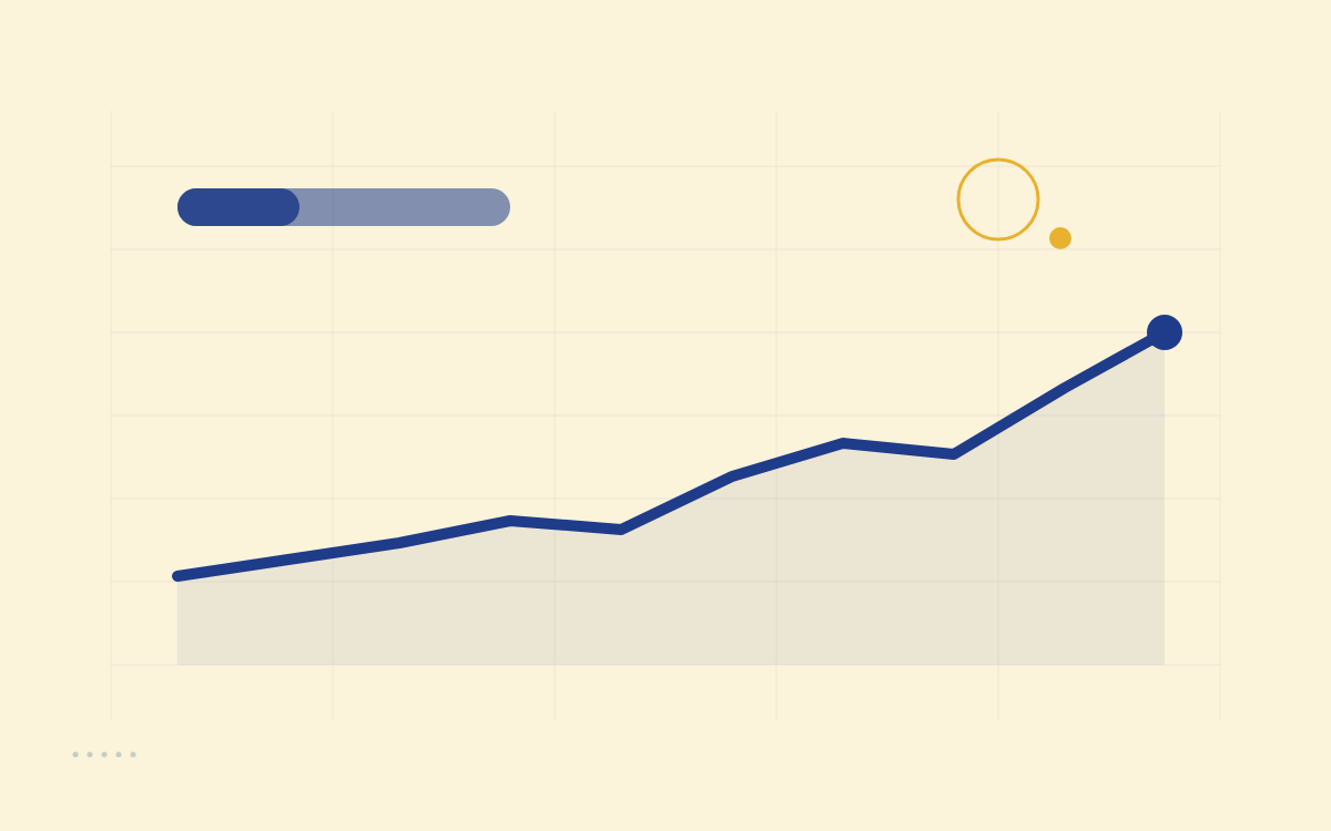
A model contributing €100 a month in constant purchasing power to the MSCI World index from January 2003 to September 2026 ends with about €87,300, against €28,500 contributed. Doubling every contribution produces twice the balance, about €174,600. All amounts are expressed in September 2026 euros; this is a historical calculation before investor taxes and fund fees.

Regular investing built capital in this example, but the outcome depended on remaining invested through market losses. A useful growth objective must account for the sequence of gains and losses, as well as the ability to keep contributing.

Key takeaways

• Contributions are a direct source of private capital. Doubling every contribution doubled the final balance under the same market path.
• Compounded growth is the relevant return measure. An arithmetic average can hide the damage losses do to a balance.
• Time alone did not remove investment risk. About 15% of forty-year single-country windows ended below contributions after inflation, making concentration and downside scenarios part of the analysis.

The recent example

The calculation uses MSCI World net total returns in euros and euro area consumer prices. Each contribution enters at month end and buys the same amount in real terms. Of the final €87,300 balance, about €58,800 comes from returns after inflation. This reflects one period in developed-market equities, including its market falls and recovery. It does not establish what a new contributor will earn.

The long-run comparison

We used annual stock-market total returns and consumer prices from the Jordà-Schularick-Taylor Macrohistory Database, release 6. This separate sample covers 13 European countries, with histories beginning between 1871 and 1900 and ending in 2020. Its single-country portfolios and longer horizons differ from the recent global-index example; the two datasets are not joined.

A hypothetical saver receives constant purchasing-power income, contributes a fixed share at each year end and spends the rest. The portfolio holds the home country’s equities, measured in local currency and deflated by local inflation. It starts with no assets and incurs no fees or taxes.

Each test requires a complete sequence of annual observations. The time-to-threshold calculation uses 1,059 sixty-year country-periods; the forty-year wealth calculation uses 1,319. The windows overlap, and the countries have different numbers of usable observations. They are not independent trials or equally weighted country averages.

Years to the spending threshold

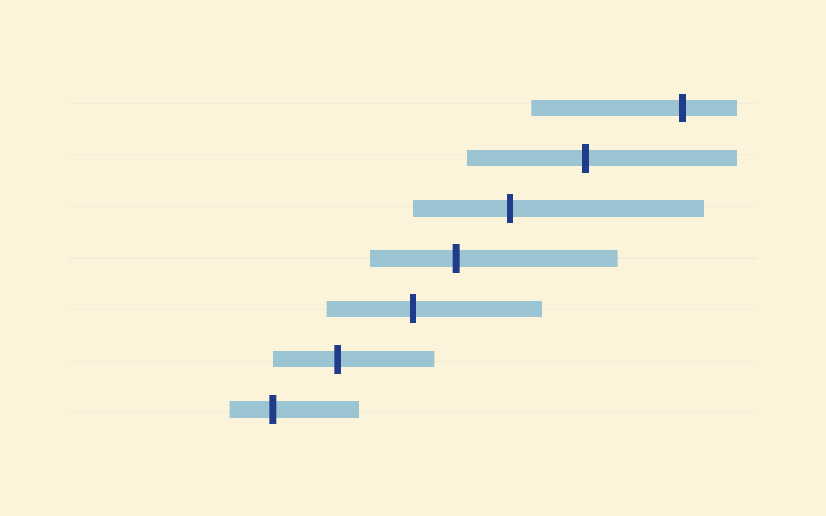
The median is 55 years at a 10% contribution rate and 39 years at 20%. Each line spans the 10th to 90th percentile. At 10% saved, 61% of windows reached the threshold within sixty years. At 20%, 93% did. Windows that failed to reach it remain in the calculation rather than being discarded.

At a 30% contribution rate, the 90th-percentile time was 42 years, compared with 46 years at the median for a 15% rate. That comparison holds for those percentiles in this sample. It does not establish that saving more always outweighs poor returns.

The threshold also moves. A 10% saver spends 90% of pay, so 25 times spending is 22.5 years of pay. A 30% saver spends 70%, making the threshold 17.5 years of pay. Part of the shorter time therefore comes from the lower assumed spending, not just a larger portfolio.

Reaching this balance does not establish retirement readiness. The experiment contains no withdrawals and does not test the often-cited 4% rule.

Forty years still produced losses

The median forty-year balance was 2.53 times total contributions after inflation. About 15% of windows finished below contributions. Among the 416 windows starting in 1950 or later, the share was 1.9%. Both figures depend on the selected markets and periods.

The earlier sample includes wars, inflation and market disruption. Recorded index returns assume that contributions and reinvestment remained possible; they cannot fully represent market closures, capital controls or an individual investor’s access. The results therefore describe a calculation on historical series, not every experience of investing through those events.

Why losses change compounded growth

Consider two hypothetical years with no contributions, withdrawals, taxes or fees. A 50% gain followed by a 50% loss turns €100 into €150 and then €75. The arithmetic average return is zero, but the annualised compounded return is -13.4%. A 50% loss requires a 100% gain to recover the starting balance before costs or withdrawals. These are arithmetic examples, not market forecasts.

Geometric growth measures the rate at which the balance compounds across all periods. For a positive balance without cash flows, it equals the ending balance divided by the starting balance, raised to one divided by the number of years, minus one. The contribution examples above add money over time, so dividing their final wealth by total contributions does not give a CAGR.

What to examine before chasing a higher return

A growth-oriented private investment plan needs a way to survive losses as well as participate in gains. The historical spread makes three checks useful:

• Contribution continuity: examine whether contributions depend on income that could fall during a market downturn.
• Concentration and liquidity: identify overlapping exposures and spending or debt commitments that could require sales during a crash.
• Growth after costs and stress: compare compounded outcomes with inflation, fees and adverse scenarios on a consistent basis.

Diversification can reduce dependence on one company or market, but broad markets can still fall together. Reducing volatility can also sacrifice expected returns; minimising risk alone does not maximise growth. A claim of “optimal” geometric growth needs explicit return assumptions, constraints and tests beyond the data used to choose the portfolio. These histories establish neither a future optimum nor a reliable way to time crashes.